Meanshift Algorithm for Image Processing

Pre-requisites - Basic idea of matrices(wrt pixels), a kernel or convolution matrix, local binary patterns, high-school statistics principles and enthu!
One of the most common and important applications of Image Processing remains Edge-Detection. The ‘algorithm’ followed for Canny-edge Detection is as follows:

• Apply a suitable filter to smooth the image in order to remove the noise
• Find the intensity gradients of the image
• Apply non-maximum suppression to get rid of spurious response to edge detection
• Apply double threshold to determine potential edges
• Track edge by hysteresis: Finalize the detection of edges by suppressing all the other edges that are weak and not connected to strong edges

As you can see, the most very first step involves filtering and removal of the noise.
WHAT IS THIS NOISE? In the sense used here, noise refers to subtle variations in pixel definitions, that may be recognised as an edge, but is most certainly not one. In the same sense as signals, it is unwanted in this purpose and needs to reduced.

The Statistics

The algorithm, in simple words, involves replacing each pixel definition with one obtained by applying the kernel on it - in general, forming a sort of mean application - which is similar to averaging out and minimising the noise.

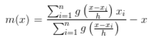
Here, g refers to the Kernel operation applied on each element Xi, where X is an assumed mean and h is a parameter called resolution. The obtained expression m(x) is referred to as the Mean Shift, on following this procedure for a large number of times, this m(x) converges to zero. We wish to minimise this m(x), without losing much information, so that further techniques of gradient can be applied for edge-detection. This is similar to Jacobi’s Method of iteration.

The Algorithm

Now, coming to the real application part of the algorithm, this method involves applying a suitable convulation matrix to the image matrix to smoothen out the edges. This matrix can be of various types, and optimised for better results. Some simple types include:

1. Flat Kernel (linear)
2. Gaussian Kernel (exponential)
3. Epanechikov Kernel (quadratic)

The simplest of these is the Flat Kernel, in which the pixel’s value is changed to the averaged value of it’s surroundings, with equal weight to each pixel.

A sample code for this algorithm, implemented in ‘MATLAB’, is as follows:

	it = 10000; %set the number of iterations of the algorithm
	for k = 1:it
    	for i = 2:nx-2
        	for j = 2:ny-2
            	Vt(i,j) = (V(i+1,j) + V(i,j+1) + V(i-1,j) + V(i,j-1))/4; % Kernel Definition
        	end        
    	end
    	V=Vt;
	end

Here, V is the image matrix of ‘nx X ny’ and Vt is a dummy matrix of same size, used during the loop. The filter can be changed by altering the line marked as Kernel Definition. Basically, the algorithm can be used to merge modes and generate clusters.

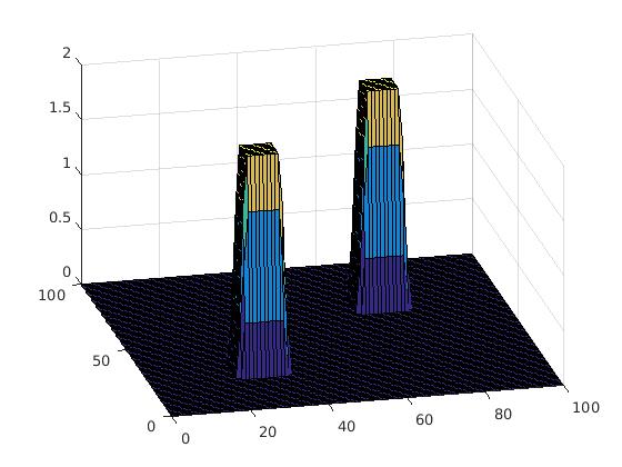
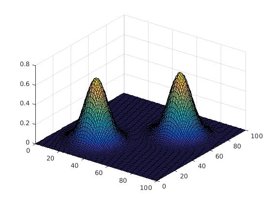
• Modes- Modes refer to the peaks in color intensities in the pixel map. When plotted, these are the peaks in ‘3D-plot’.
• Clusters- Clusters refer to the groups of similarly defined pixels, ie, groups with similar color or compositon.

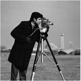
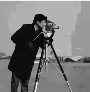
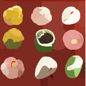
As you can see in the images below, as the number of iterations increase, modes get merged and a cluser is formed.

THE PARAMETERS: The alterable parameters include: *‘it’ or the number of iterations. Increasing ‘it’ would increase the merge rate, but also increase the computational cost as number of iterations would increase. Hence, there is an optimised upper bound for this value.

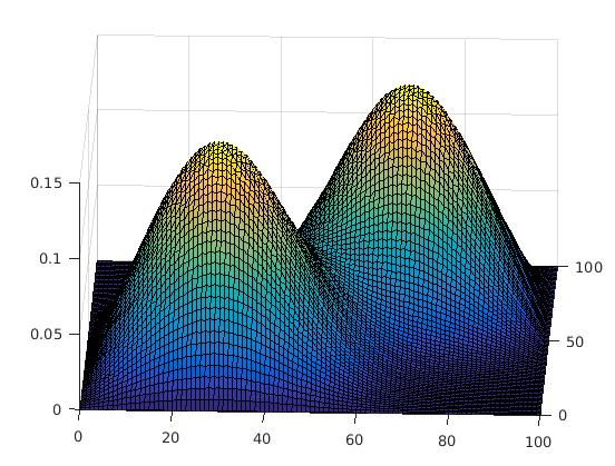
*‘h’ or resolution is a parameter used in the statistical definition. Since it is in the denominator, it can play a huge role in the smoothening effect as shown. In general, a large ‘h’ would mean faster convergence, larger clusters and more loss of information. This value can be tweaked as desired, for optimal results.

For more such example, you can refer to this PDF.

ADVANTAGES Comparing with other clustering algo K-means, it does not ASSUME any cluster etc. and the algo ensures that clusters are sorted automatically. Also, it is robust and works for any no. of (non-predefined) modes.

DRAWBACKS The iterative technique is highly redundant and computationally expensive; also, the method doesnt work well in free space (3D), as there may exist many local maximas that converge to optimas and mode isolation cannot be done.

This concludes the summary of an essential algorithm in the art of Image Processing. Hope you enjoyed it!

• ← Previous Post
• Next Post →